
Increasing DataLoader workers made this FashionMNIST training loop faster. I used torch.profiler to see where the time was going. With random cropping and rotation on the CPU, the zero-worker loop spent a long time obtaining each batch. Four worker processes shortened that wait.
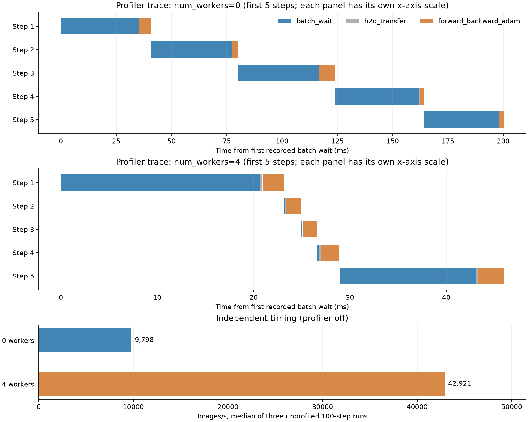
With the profiler removed, throughput rose from about 9,798 to 42,921 images/s—roughly 4.4 times as fast. The trace explains where to look; the separate timing run measures the speed difference without the profiler’s recording overhead.
The long interval was the next batch
| Unprofiled measurement: three runs of 100 steps | 0 workers | 4 workers |
|---|---|---|
| Median throughput | 9,798 images/s | 42,921 images/s |
| Median time for 100 steps | 2.613 s | 0.596 s |
Median of the three per-run median next(DataLoader) waits |
23.781 ms | 0.169 ms |
Both conditions used batches of 256, so 100 steps processed 25,600 images. The script ran 40 warm-up steps first; worker startup is not included in this table. Reversing the execution order for the middle repetition did not change which condition was faster.
next(DataLoader) is the call that retrieves the next batch. With no workers, the training process itself performs the crop, rotation and tensor conversion. With four workers, separate processes can prepare batches ahead of time.
The batch wait can overlap GPU work. Do not add its duration to the other intervals and treat the sum as total training time. Throughput was measured separately, after waiting for CUDA work to finish.
The 20-step profiler recording gave different batch-wait medians: 35.952 ms for zero workers and 0.116 ms for four. Recording CPU and CUDA activity adds overhead. Even the four-worker trace had occasional waits: its 95th percentile was 16.621 ms. Parallel loading did not remove every stall.
What was running
The PC used a Core i7-14700F and an RTX 5070 Ti with 16 GB of VRAM. The environment was Windows 11, WSL 2 with Ubuntu 26.04 LTS, PyTorch 2.13.0+cu130 and torchvision 0.28.0+cu130.
The two conditions shared the FashionMNIST training set, CNN, initial weights, batch size 256, seed 42, FP32 with TF32 disabled, and pin_memory=True. Preprocessing was RandomResizedCrop(28, scale=(0.75, 1.0)), RandomRotation(15) and ToTensor. The four-worker condition used persistent_workers=True and prefetch_factor=2.
This compares waiting time under that preprocessing workload, not model accuracy. It also does not predict the benefit for a loader that only applies ToTensor, or for a much larger model whose GPU computation dominates each step.
Run it from the repository
You need CUDA-enabled PyTorch and a compatible torchvision installation. FashionMNIST downloads about 31 MB of compressed data. Allow at least 300 MB for data and results in addition to the Python environment: the zero-worker trace alone was about 106 MB. With the GPU environment already working, the experiment took about a minute excluding downloads and required no restart or administrator privileges.
git clone https://github.com/matrizea/yuyuyuroom-ai-experiments.git ~/ai-experiments
cd ~/ai-experiments
python -c 'import torch; print(torch.cuda.is_available())'
python -m pip install matplotlib numpy
python ai_lab/experiment_training_profiler.py
python ai_lab/plot_training_profiler.py
python -m unittest discover -s ai_lab -p test_training_profiler.py -v
~/ai-experiments is an example checkout location. If the CUDA check prints False, fix the GPU environment before comparing workers. Use the PyTorch installation selector if PyTorch or torchvision is missing. The WSL GPU setup article (Japanese) covers the local setup used here.
The script writes to ai_lab/results/training_profiler/: result.json, timed_steps_raw.csv with all 600 measured steps, two trace files (workers_0_trace.json and workers_4_trace.json), and operator tables. The tests finish with Ran 3 tests ... OK. The chart is written to figures/pytorch-profiler-dataloader-wait.png. Another PC will produce different times; first check that both traces and the result files were generated.
Label the operations you want to distinguish
The script uses record_function to mark three intervals:
with profile(activities=[ProfilerActivity.CPU, ProfilerActivity.CUDA]) as prof:
    for _ in range(20):
        with record_function("batch_wait"):
            batch = next(iterator)
        with record_function("h2d_transfer"):
            images, labels = (x.to("cuda", non_blocking=True) for x in batch)
        with record_function("forward_backward_adam"):
            optimizer.zero_grad(set_to_none=True)
            loss = loss_fn(model(images), labels)
            loss.backward()
            optimizer.step()
        prof.step()
batch_wait covers the CPU call that requests a batch. h2d_transfer covers submitting the host-to-GPU transfer. The final interval includes prediction, gradient calculation and the optimizer update. CUDA calls are asynchronous, so the length of a CPU-side interval is not automatically the GPU’s execution time.
Both traces also contained 940 CUDA kernel events. In the chart, the zero-worker batch wait occupies much of each step. Four workers shorten it in most of the displayed steps, though the first and fifth still contain a wait. The horizontal scales differ, so use the unprofiled table—not the visual width of the rows—to compare speed.
The PyTorch profiler documentation explains the activity records and trace export. If CUDA activity is absent despite requesting ProfilerActivity.CUDA, check PyTorch’s GPU setup and whether the profiling environment can use CUPTI; successful GPU computation alone does not guarantee a complete trace.
Measure speed again without the profiler
The large trace records many small CPU preprocessing operations. Reporting its elapsed time as ordinary training speed would include the cost of observing the program.
For the speed table, profiling was disabled and torch.cuda.synchronize() waited for outstanding GPU work at the end of each 100-step run. The workers were already warm. Short jobs can spend a substantial fraction of their time starting processes, so these numbers should not be used as total time from launch to completion. The worker-count experiment (Japanese) includes startup behavior.
Here the trace located the wait, and the separate timing run confirmed that moving preprocessing into worker processes helped. Those are useful checks to keep separate when changing a training loop.