
HOG features with a linear SVM reached 88.85% accuracy on FashionMNIST, ahead of 87.00% for a small CNN trained for three epochs. The CNN was much faster on the GPU, though. Extracting HOG features was particularly expensive at prediction time.
This comparison uses the same 60,000 training images and 10,000 test images. It is a comparison of two specific configurations on one PC—not an upper limit on CNN accuracy.
Accuracy favored HOG; runtime favored the GPU CNN
| Measurement | HOG + Linear SVM, CPU | CNN, GPU, 3 epochs |
|---|---|---|
| Test accuracy | 88.85% | 87.00% |
| Training-image feature extraction | 13.73 s | Part of training |
| Training | 50.45 s | 3.59 s |
| Test preprocessing and inference | About 2.25 s | 0.142 s |
The CPU was a Core i7-14700F; the GPU was an RTX 5070 Ti. The timings therefore include different processors as well as different methods. HOG extraction plus SVM fitting took 64.18 seconds.
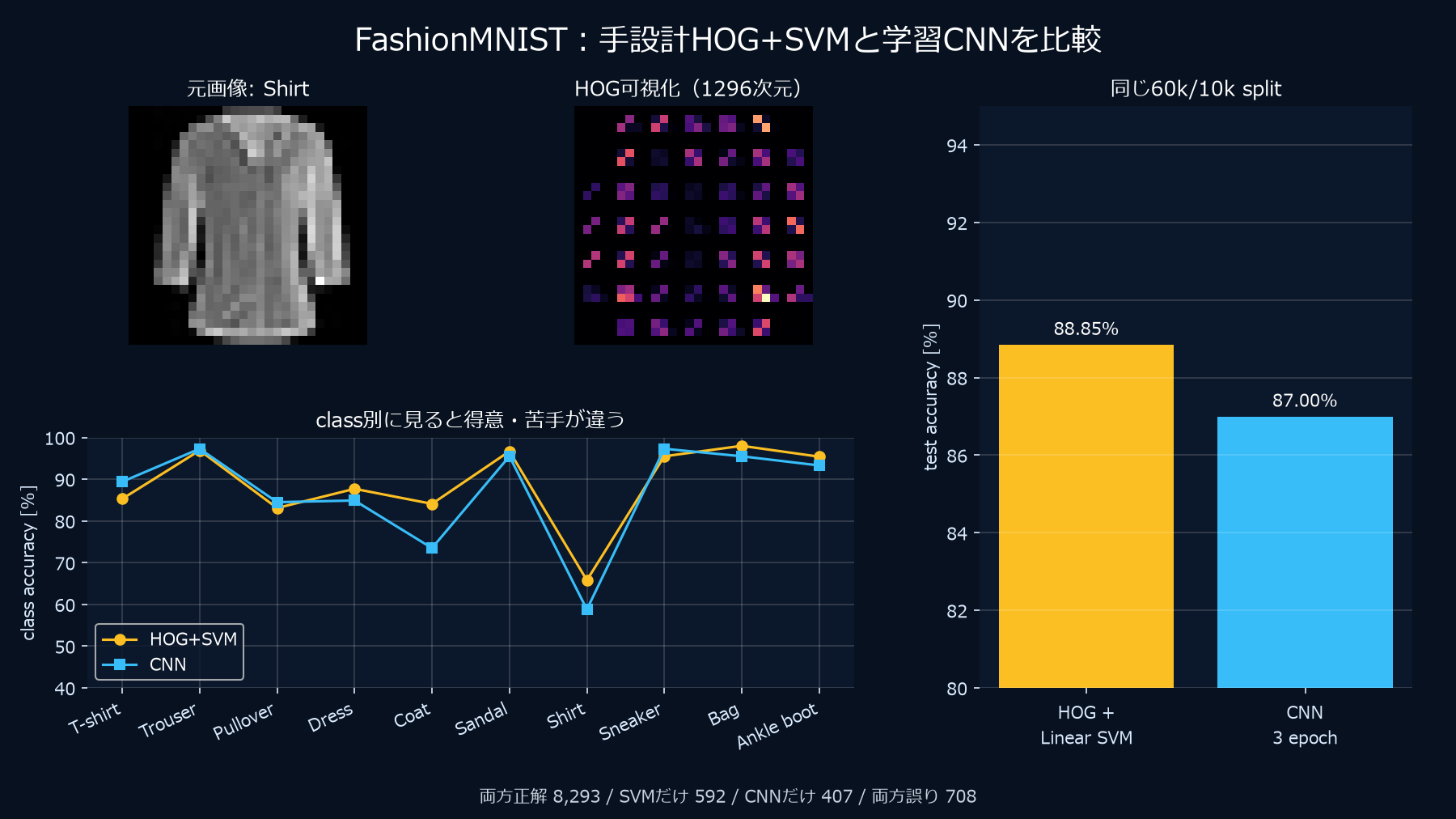
What HOG extracts from the image
HOG stands for Histogram of Oriented Gradients. It describes the directions of local brightness changes rather than using pixel values directly. Sleeves, shoe soles and bag outlines produce strong gradients at their edges.
For horizontal and vertical brightness differences gx and gy, the gradient magnitude and direction are:
magnitude = sqrt(gx² + gy²)
angle     = atan2(gy, gx)
The image is split into small cells. Each cell collects a histogram of gradient directions, weighted by gradient magnitude. The configuration was:
features = hog(
    image,
    orientations=9,
    pixels_per_cell=(4, 4),
    cells_per_block=(2, 2),
    block_norm="L2-Hys",
)
A 28×28 image contains 7×7 cells of 4×4 pixels. A 2×2-cell block can occupy 6×6 positions when it moves one cell at a time. Each block contributes 2 × 2 × 9 = 36 values, giving 6 × 6 × 36 = 1,296 features.
The feature vector is larger than the original 784-pixel image. HOG is not dimensionality reduction here: overlapping normalized blocks repeat information while reducing sensitivity to local contrast changes. Storing all 60,000 vectors as float32 takes about 296.6 MiB, before the classifier’s other allocations. The scikit-image HOG example illustrates the extraction stages.
The classifier and CNN
The SVM uses the HOG vectors as input:
svm = LinearSVC(
    C=1.0,
    dual="auto",
    max_iter=5000,
    random_state=42,
)
svm.fit(hog_train, y_train)
prediction = svm.predict(hog_test)
For each class, a linear score has the form w · x + b; the classifier chooses the class with the largest score. This is LinearSVC, not an RBF-kernel SVC. The nonlinear feature construction happens before the linear classifier.
The CNN instead receives pixels scaled to 0–1 and learns its filters:
1×28×28
  → Conv 1→16 → ReLU → MaxPool
  → Conv 16→32 → ReLU → MaxPool
  → Linear 1568→64 → ReLU
  → Linear 64→10
It has 105,866 parameters and uses Adam with learning rate 0.001, batch size 256 and three epochs. No random crops or rotations were added. DataLoader used four workers and pinned memory. GPU warm-up happened before timing, and the model was recreated from the original seed afterward so the dummy update did not become part of training.
Longer training, augmentation or a different CNN could change the ranking. The 87.00% result belongs to this training budget and architecture.
The largest gap was for coats
| Class | HOG + SVM | CNN | SVM minus CNN |
|---|---|---|---|
| T-shirt/top | 85.3% | 89.4% | −4.1 percentage points |
| Trouser | 96.9% | 97.3% | −0.4 |
| Pullover | 83.1% | 84.5% | −1.4 |
| Dress | 87.7% | 84.9% | +2.8 |
| Coat | 84.1% | 73.5% | +10.6 |
| Sandal | 96.7% | 95.5% | +1.2 |
| Shirt | 65.8% | 58.8% | +7.0 |
| Sneaker | 95.5% | 97.3% | −1.8 |
| Bag | 98.0% | 95.5% | +2.5 |
| Ankle boot | 95.4% | 93.3% | +2.1 |
Of 1,000 coat images, the CNN classified 122 as pullovers and 110 as shirts. HOG + SVM made those mistakes 64 and 54 times, respectively. On T-shirt/top images, the CNN was 4.1 percentage points ahead instead.
Shirt was the hardest class for both methods. The SVM classified 130 shirts as T-shirts, 82 as pullovers and 82 as coats. The CNN counts were 211, 106 and 70. Small grayscale images of upper-body clothing can share similar outlines; the overall accuracy near 89% hides much weaker performance on shirts.
Most of the SVM prediction time was feature extraction
Extracting HOG features for 10,000 test images took 2.22 seconds. Applying the trained SVM took only 0.028 seconds. Feature preparation accounted for about 99% of the combined time.
The CNN’s 0.142-second GPU inference run was about 15.8 times faster than HOG extraction plus CPU SVM prediction. Comparing only the 0.028-second SVM call would leave out the work needed to produce its input. Conversely, this result does not tell us which method would be faster if both had to run on a CPU.
The two methods also made different mistakes. Both were correct on 8,293 images; only the SVM was correct on 592, only the CNN on 407, and both were wrong on 708. Their predicted labels agreed on 88.29% of the test set.
At least one method was correct on 9,292 images. That is a count made after looking at the labels, not a demonstrated 92.92%-accurate ensemble. A rule for choosing between the predictions would need its own training or validation data and a separate test.
Reproduce the comparison
Use a CUDA-enabled PyTorch environment in WSL 2, with compatible torchvision. The recorded run used PyTorch 2.13.0+cu130. The SVM and HOG steps run on the CPU; the script requires a CUDA GPU for the CNN rather than silently switching to a different comparison.
FashionMNIST downloads about 31 MB of compressed data. The training HOG array alone is roughly 297 MiB, so allow additional RAM for extraction, classifier fitting and the CNN. Runtime depends strongly on CPU load and GPU availability; the original feature-extraction and SVM-fit stages alone took about a minute. Existing Python environments do not require administrator access or a restart for the following commands.
git clone https://github.com/matrizea/yuyuyuroom-ai-experiments.git ~/ai-experiments
cd ~/ai-experiments
python -c 'import torch; print(torch.cuda.is_available())'
python -m pip install numpy matplotlib scikit-learn scikit-image
python ai_lab/experiment_hog_svm_vs_cnn.py \
  --data-dir ai_lab/data \
  --output ai_lab/results/hog_svm_vs_cnn.json \
  --figure figures/hog-svm-vs-cnn.png
The result JSON records hog_feature_dimension as 1296, separate extraction/fitting/prediction times, class accuracies, confusion matrices and the four correctness counts. Those four counts should add up to 10,000. Timing and CNN results may vary with software and hardware; the published tables above retain the original run rather than mixing values from different runs.
If the CUDA check prints False, use the PyTorch installation selector before starting the comparison. A dataset-download error needs a network check, not a change to the train/test split. Keep the JSON even when a result differs: it shows whether the difference is in accuracy, feature extraction or training time.